This page was generated from examples/webservices.ipynb. Interactive online version:

Web Services

from datetime import datetime

import pygeoogc as ogc
import pygeoutils as geoutils
import xarray as xr
from pygeoogc import WFS, WMS, ArcGISRESTful, ServiceURL
from pynhd import NLDI

PyGeoOGC and PyGeoUtils can be used to access any web services that are based on ArcGIS RESTful, WMS, or WFS. It is noted that although, all these web service have limits on the number of objects (e.g., 1000 objectIDs for RESTful) or pixels (e.g., 8 million pixels) per requests, PyGeoOGC takes care of dividing the requests into smaller chunks under-the-hood and then merges them.

Let’s get a watershed geometry using NLDI and use it for subsetting the data.

basin = NLDI().get_basins("11092450")
basin_geom = basin.geometry[0]

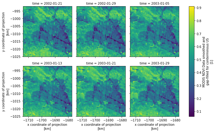
PyGeoOGC, has a function for asynchronous download which can help speed up sending/receiveing requests. For example, let’s use this function to get NDVI data from DACC server. The function can be directly passed to xarray.open_mfdataset to get the data as an xarray Dataset.

west, south, east, north = basin_geom.bounds
base_url = "https://thredds.daac.ornl.gov/thredds/ncss/ornldaac/1299"
dates_itr = ((datetime(y, 1, 1), datetime(y, 1, 31)) for y in range(2000, 2005))
urls = (
    (
        f"{base_url}/MCD13.A{s.year}.unaccum.nc4",
        {
            "var": "NDVI",
            "north": f"{north}",
            "west": f"{west}",
            "east": f"{east}",
            "south": f"{south}",
            "disableProjSubset": "on",
            "horizStride": "1",
            "time_start": s.strftime("%Y-%m-%dT%H:%M:%SZ"),
            "time_end": e.strftime("%Y-%m-%dT%H:%M:%SZ"),
            "timeStride": "1",
            "addLatLon": "true",
            "accept": "netcdf",
        },
    )
    for s, e in dates_itr
)
data = xr.open_mfdataset(ogc.async_requests(urls, "binary", max_workers=8))

data.isel(time=slice(10, 16)).NDVI.plot(x="x", y="y", row="time", col_wrap=3);

<xarray.plot.facetgrid.FacetGrid at 0x7f92460fb070>

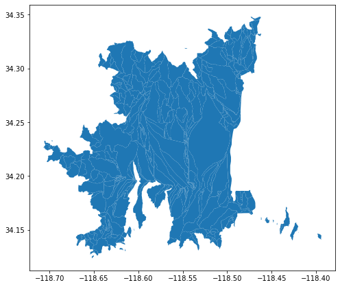
Moreover, PyGeoOGC has a NamedTuple called ServiceURL that contains URLs of the some of the popular web services. Let’s use it to access NHDPlus HR Dataset RESTful service and get all the catchments that our basin contain and use pygeoutils.json2geodf to convert it into a GeoDataFrame.

hr = ArcGISRESTful(ServiceURL().restful.nhdplushr, outformat="json")
hr.layer = 10
hr.spatial_relation = "esriSpatialRelContains"
hr.oids_bygeom(basin_geom, "epsg:4326")
resp = hr.get_features()
catchments = geoutils.json2geodf(resp)

576 features found in the requested region.

catchments.plot(figsize=(8, 8));

<AxesSubplot:>

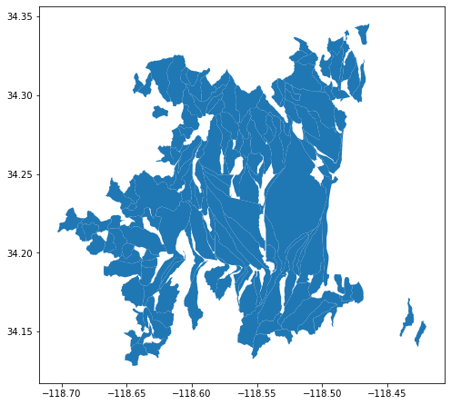
Note oids_bygeom has an additional argument for passing any valid SQL WHERE clause to further filter the data on the server side. For example, let’s only keep the ones with an area of larger than 0.5 sqkm.

hr.oids_bygeom(basin_geom, geo_crs="epsg:4326", sql_clause="AREASQKM > 0.5")
resp = hr.get_features()
catchments = geoutils.json2geodf(resp)

148 features found in the requested region.

catchments.plot(figsize=(8, 8));

<AxesSubplot:>

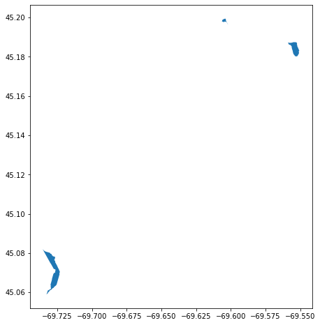
We can also submit a query based on IDs of any valid field in the database. If the measure property is desired you can pass return_m as True to the get_features class method:

hr.oids_byfield("NHDPLUSID", [5000500013223, 5000400039708, 5000500004825])
resp = hr.get_features(return_m=True)
catchments = geoutils.json2geodf(resp)

3 features found in the requested region.

catchments.plot(figsize=(8, 8));

<AxesSubplot:>

Next, let’s get wetlands using the National Wetlands Inventory WMS service. First we need to connect to the service using WMS class.

wms = WMS( ServiceURL().wms.fws, layers="1", outformat="image/tiff", crs="epsg:3857", )

Then we can get the data using the getmap_bybox function. Note that this function only accpets a bounding box, so we need to pass a bounding box and mask the returned data later on usin pygeoutils.gtiff2xarray function.

r_dict = wms.getmap_bybox( basin_geom.bounds, 1e3, box_crs="epsg:4326", ) wetlands = geoutils.gtiff2xarray(r_dict, basin_geom, "epsg:4326")

There are three bands in the returned data. Using the information provided for the layer here we can find the color code of emergent wetlands and extract them.

emergent = [127, 195, 28] wl_emergent = wetlands.where( (wetlands.isel(band=0) == emergent[0]) & (wetlands.isel(band=1) == emergent[1]) & (wetlands.isel(band=2) == emergent[2]) )

For plotting the wetlands note that in our request we set the CRS to EPSG:3857 so we need transform the watershed geometry to this CRS so they can be superimposed.

basin_3857 = basin.to_crs("epsg:3857") ax = basin_3857.plot(facecolor="none", edgecolor="k", lw=0.5, figsize=(8, 8)) wl_emergent.isel(band=0).plot(ax=ax, add_colorbar=False);

Next, let’s getthe base flood elevation data from FEMA and use pygeoutils.json2geodf to convert it into a GeoDataFrame.

wfs = WFS(
    ServiceURL().wfs.fema,
    layer="public_NFHL:Base_Flood_Elevations",
    outformat="esrigeojson",
    crs="epsg:4269",
)

wfs

Connected to the WFS service with the following properties:
URL: https://hazards.fema.gov/gis/nfhl/services/public/NFHL/MapServer/WFSServer
Version: 2.0.0
Layer: public_NFHL:Base_Flood_Elevations
Output Format: esrigeojson
Output CRS: epsg:4269

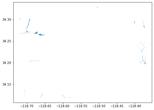
r = wfs.getfeature_bybox(basin_geom.bounds, box_crs="epsg:4326")
flood = geoutils.json2geodf(r.json(), "epsg:4269", "epsg:4326")
flood.plot(figsize=(8, 8));

<AxesSubplot:>

WFS also supports any valid CQL filter.

layer = "wmadata:huc08"
wfs = WFS(
    ServiceURL().wfs.waterdata,
    layer=layer,
    outformat="application/json",
    version="2.0.0",
    crs="epsg:4269",
)
r = wfs.getfeature_byfilter(f"huc8 LIKE '13030%'")
huc8 = geoutils.json2geodf(r.json(), "epsg:4269", "epsg:4326")

huc8.plot(figsize=(8, 8));

<AxesSubplot:>